Benchmark problems

smt-optim comes with many test problems for benchmarking. This notebook shows how to get the problems, filter them and plot them.

import numpy as np
import matplotlib.pyplot as plt

from smt_optim.benchmarks.registry import list_problems

Overview

The list_problems method allows us to retrieve a list of BenchmarkProblem problems with specific attributes. If no attributes are given, it will return all the problems implemented in smt-optim. The example below, first all problems are fetch. Then only problems of dimension 2 present in the SFU collection are fetched. The parameter n, which corresponds to the number of variable, expects a lower and upper bound.

problems = list_problems()
print("Number of problem found:", len(problems))

problems = list_problems(n=[2, 2], tags=["sfu"])
print("Number of problem found:", len(problems))

Number of problem found: 36
Number of problem found: 10

The BenchmarkProblem class has several key attributes:

• num_dim: The number of dimensions

• num_obj: The number of objectives

• num_cstr: The number of constraints

• num_fidelity: The number of fidelity levels (for multi-fidelity problems)

• bounds: The variable bounds

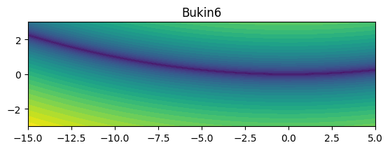
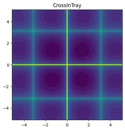
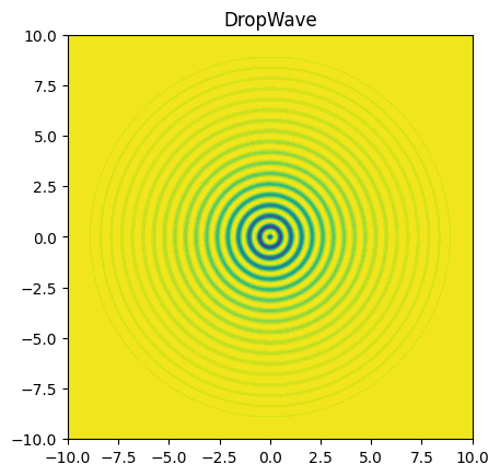
For mono-fidelity BenchmarkProblems, the objective function can be evaluated using the objective class method. Here’s an example code snippet that plots 3 problems on their respective domains:

num_display = 3

for idx, prob in enumerate(problems):
    X = np.linspace(prob.bounds[0, 0], prob.bounds[0, 1], 201)
    Y = np.linspace(prob.bounds[1, 0], prob.bounds[1, 1], 201)
    XX, YY = np.meshgrid(X, Y)

    data = np.vstack((XX.ravel(), YY.ravel())).T
    z = np.empty(data.shape[0])

    for i in range(data.shape[0]):
        z[i] = prob.objective(data[i, :])

    Z = z.reshape(XX.shape)

    fig, ax = plt.subplots()
    ax.contourf(XX, YY, Z, levels=30)
    ax.set_title(prob.name)
    ax.set_aspect('equal')

    plt.show()

    if idx+1 >= num_display:
        break

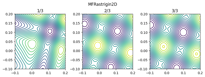
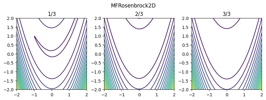
Multi-fidelity Benchmark Problems

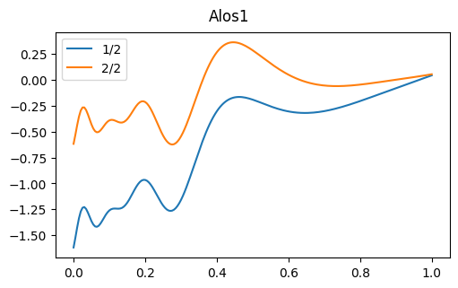
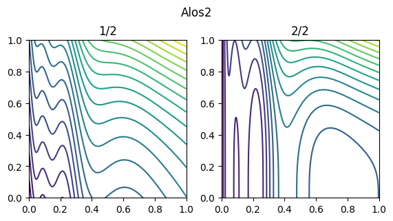
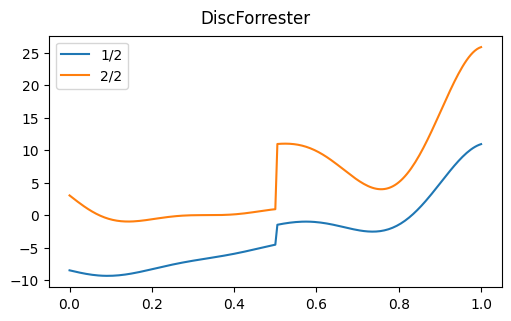
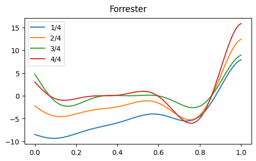
The code snippet below retrieves and plots all 1D and 2D multi-fidelity analytical benchmark problems from the AVT-311 L1 benchmarks. Note that for multi-fidelity problems, the objectives attribute returns a list of callable objective functions in increasing order of fidelity.

problems = list_problems(n=[1, 2], tags=["avt311"])
print("Number of problem found:", len(problems))

for prob in problems:

    if prob.num_dim == 1:

        fig, ax = plt.subplots(layout="constrained", figsize=(5, 3.1))
        fig.suptitle(prob.name)
        x = np.linspace(prob.bounds[0, 0], prob.bounds[0, 1], 201)

        for lvl in range(prob.num_fidelity):
            z = np.empty_like(x)

            for idx in range(x.shape[0]):
                z[idx] = prob.objectives[lvl](x[idx])

            ax.plot(x, z, label=f"{lvl+1}/{prob.num_fidelity}")

        ax.legend()
        plt.show()

    elif prob.num_dim == 2:
        X = np.linspace(prob.bounds[0, 0], prob.bounds[0, 1], 201)
        Y = np.linspace(prob.bounds[1, 0], prob.bounds[1, 1], 201)
        XX, YY = np.meshgrid(X, Y)

        data = np.vstack((XX.ravel(), YY.ravel())).T
        z = np.empty(data.shape[0])

        fig, ax = plt.subplots(1, prob.num_fidelity, layout="constrained", figsize=(2.8*prob.num_fidelity, 3.1))
        fig.suptitle(prob.name)

        for lvl in range(prob.num_fidelity):
            for i in range(data.shape[0]):
                z[i] = prob.objectives[lvl](data[i, :])
            Z = z.reshape(XX.shape)
            ax[lvl].contour(XX, YY, Z, levels=20)
            ax[lvl].set_title(f"{lvl+1}/{prob.num_fidelity}")
            # ax[lvl].set_aspect('equal')

        plt.show()

Number of problem found: 6