Mutli-fidelity optimization - MFSEGO#
import numpy as np
from matplotlib import pyplot as plt

from smt_optim.benchmarks.registry import get_problem

from smt_optim.core import Driver, ObjectiveConfig, ConstraintConfig, DriverConfig, Problem

from smt_optim.surrogate_models.smt import SmtAutoModel

from smt_optim.acquisition_strategies import MFSEGO

import scipy.optimize as so
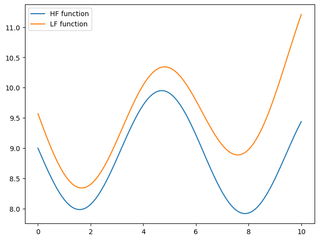
Unconstrained 1D optimization#
# high-fidelity function
def sasena2002_hf(x):
    return -np.sin(x) - np.exp(x / 100) + 10

# low-fidelity function
def sasena2002_lf(x):
    return sasena2002_hf(x) + 0.3 + 0.03 * (x - 3) ** 2

bounds = np.array([[0, 10]])

x_valid = np.linspace(bounds[:, 0], bounds[:, 1], 101)
y_hf = sasena2002_hf(x_valid)
y_lf = sasena2002_lf(x_valid)

fig, ax = plt.subplots(layout="constrained")
ax.plot(x_valid, y_hf, label="HF function")
ax.plot(x_valid, y_lf, label="LF function")

plt.legend()
plt.show()
obj_config = ObjectiveConfig(
    objective=[sasena2002_lf, sasena2002_hf],   # multi-fidelity functions must be given in sequential order
    type="minimize",
    surrogate=SmtAutoModel,
)


prob_definition = Problem(
    obj_configs=[obj_config],
    design_space=bounds,
    costs=[0.2, 1],                 # Set the cost of sampling each level
)


opt_config = DriverConfig(
    max_iter = 10,
    max_budget = 10,                # stopping criterion
    nt_init = 3,
    verbose = True,
    scaling = True,
    seed=42,
)

driver = Driver(prob_definition, opt_config, MFSEGO)

state = driver.optimize()
          iter         budget           fmin           rscv       fidelity        gp_time       acq_time
             1          4.400    7.98412e+00      0.000e+00              1          0.130          0.124
             2          4.600    7.98412e+00      0.000e+00              1          0.118          0.170
             3          5.800    7.98412e+00      0.000e+00              2          0.127          0.142
             4          6.000    7.98412e+00      0.000e+00              1          0.165          0.295
             5          7.200    7.91824e+00      0.000e+00              2          0.187          0.229
             6          8.400    7.91824e+00      0.000e+00              2          0.176          0.246
             7          9.600    7.91824e+00      0.000e+00              2          0.176          0.219
             8         10.800    7.91824e+00      0.000e+00              2          0.194          0.261
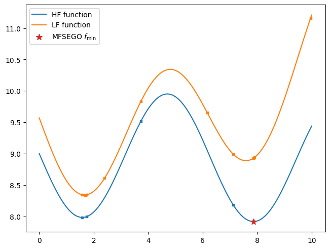
data = state.dataset.export_as_dict()
fidelity_masks = [(data["fidelity"] == lvl).ravel() for lvl in range(state.problem.num_fidelity)]
xt = [data["x"][fidelity_masks[lvl], 0] for lvl in range(state.problem.num_fidelity)]
yt = [data["obj"][fidelity_masks[lvl], 0] for lvl in range(state.problem.num_fidelity)]
sample = state.get_best_sample()

fig, ax = plt.subplots(layout="constrained")
ax.plot(x_valid, y_hf, label="HF function")
ax.plot(x_valid, y_lf, label="LF function")

for lvl in reversed(range(2)):
    ax.scatter(xt[lvl], yt[lvl], 5, marker="s")

ax.scatter(sample.x, sample.obj, 75, marker="*", color="C3", zorder=20, label=r"MFSEGO $f_{\min}$")

plt.legend()
plt.show()
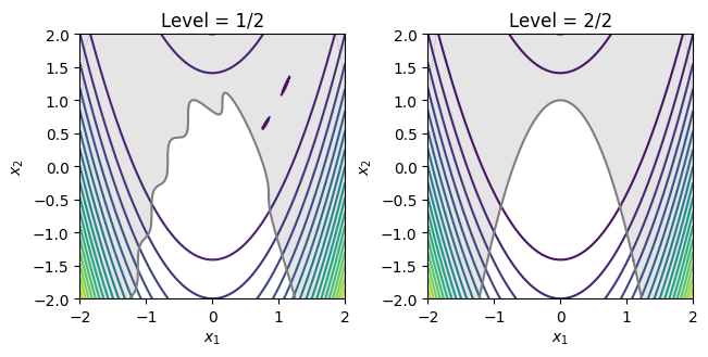
Constrained 2D optimization#
Importing a test function#
problem = get_problem("Rosenbrock")

X = np.linspace(problem.bounds[0, 0], problem.bounds[0, 1], 201)

XX, YY = np.meshgrid(X, X)

data = np.vstack((XX.ravel(), YY.ravel())).T
z = np.empty(data.shape[0])
c = np.empty(data.shape[0])

fig, ax = plt.subplots(1, 2, layout="constrained")

for lvl in range(2):

    ax[lvl].set_title(f"Level = {lvl+1}/2")

    for i in range(data.shape[0]):
        z[i] = problem.objective[lvl](data[i, :])
        c[i] = problem.constraints[0][lvl](data[i, :])

    Z = z.reshape(XX.shape)
    C = c.reshape(XX.shape)

    ax[lvl].contour(XX, YY, Z, levels=20)

    ax[lvl].contourf(XX, YY, np.where(C <= 0, np.nan, C), levels=0, colors="C7", alpha=0.20)
    ax[lvl].contour(XX, YY, C, levels=[0], colors="C7")

    ax[lvl].set_xlabel(r"$x_1$")
    ax[lvl].set_ylabel(r"$x_2$")
    ax[lvl].set_aspect("equal")

plt.show()
MFSEGO Configuration#
obj_config = ObjectiveConfig(
    problem.objective,
    type="minimize",
    surrogate=SmtAutoModel,

)

# configure the constraint
cstr_config = ConstraintConfig(
    problem.constraints[0],
    upper=0.0,                      # g(x) <= 0
    surrogate=SmtAutoModel,         # set which GP to model this constraint
)


prob_definition = Problem(
    obj_configs=[obj_config],
    design_space=problem.bounds,
    costs=[0.5, 1],                 # Set the cost of sampling each level
    cstr_configs=[cstr_config],
)


opt_config = DriverConfig(
    max_iter = 20,
    max_budget = 60,                # stopping criterion
    nt_init = 5,
    verbose = True,
    scaling = True,
    seed=0,
)

strategy_kwargs = {
    "n_start": 20,
    "fidelity_crit": "pessimistic",     # fidelity selection criterion
    "sp_method": "Cobyla",              # SciPy optimizer method
    "sp_tol": 1e-4,                     # SciPy optimizer tolerance
}

driver = Driver(prob_definition, opt_config, MFSEGO, strategy_kwargs=strategy_kwargs)

state = driver.optimize()
          iter         budget           fmin           rscv       fidelity        gp_time       acq_time
             1         10.500    2.64887e+00      0.000e+00              1          0.916          1.862
             2         11.000    2.64887e+00      0.000e+00              1          0.739          1.415
             3         11.500    2.64887e+00      0.000e+00              1          0.733          1.277
             4         12.000    2.64887e+00      0.000e+00              1          0.667          1.192
             5         12.500    2.64887e+00      0.000e+00              1          0.708          2.169
             6         13.000    2.64887e+00      0.000e+00              1          0.774          2.446
             7         13.500    2.64887e+00      0.000e+00              1          0.759          2.714
             8         14.000    2.64887e+00      0.000e+00              1          0.750          2.796
             9         14.500    2.64887e+00      0.000e+00              1          0.760          2.832
            10         15.000    2.64887e+00      0.000e+00              1          0.839          2.334
          iter         budget           fmin           rscv       fidelity        gp_time       acq_time
            11         15.500    2.64887e+00      0.000e+00              1          0.743          2.530
            12         16.000    2.64887e+00      0.000e+00              1          0.804          2.711
            13         16.500    2.64887e+00      0.000e+00              1          0.987          2.285
            14         18.000    2.64887e+00      0.000e+00              2          0.820          1.839
            15         19.500    2.78736e-01      0.000e+00              2          0.695          1.442
            16         20.000    2.78736e-01      0.000e+00              1          0.617          2.431
            17         21.500    1.79294e-01      0.000e+00              2          0.602          2.235
            18         23.000    1.78500e-01      2.982e-05              2          0.632          2.746
            19         24.500    1.78479e-01      1.487e-05              2          0.618          2.799
            20         26.000    1.78479e-01      1.487e-05              2          0.683          2.711
Validation with SLSQP#
SLSQP is a mono-fidelity gradient-based solver.
cstrs = [{
        "fun": lambda x, f=problem.constraints[0][-1]: -f(x),
        "type": "ineq",
        }]

res = so.minimize(problem.objective[-1], [0.5, 0.5], bounds=problem.bounds, constraints=cstrs, method="SLSQP", tol=1e-15)

print(res)
     message: Optimization terminated successfully
     success: True
      status: 0
         fun: 0.17848414871339022
           x: [ 5.777e-01  3.325e-01]
         nit: 6
         jac: [-5.631e-01 -2.437e-01]
        nfev: 19
        njev: 6
 multipliers: [ 4.873e-01]
data_x = []
for lvl in range(state.problem.num_fidelity):
samples = state.dataset.get_by_fidelity(lvl)
data_x.append(np.empty((len(samples), state.problem.num_dim)))
for idx, s in enumerate(samples):
data_x[lvl][idx, :] = s.x
sample = state.get_best_sample(ctol=1e-4)
print(f"best sample = \n{sample}")
X = np.linspace(problem.bounds[0, 0], problem.bounds[0, 1], 201)
XX, YY = np.meshgrid(X, X)
data = np.vstack((XX.ravel(), YY.ravel())).T
z = np.empty(data.shape[0])
c = np.empty(data.shape[0])
for i in range(data.shape[0]):
z[i] = problem.objective[-1](data[i, :])
c[i] = problem.constraints[0][-1](data[i, :])
Z = z.reshape(XX.shape)
C = c.reshape(XX.shape)
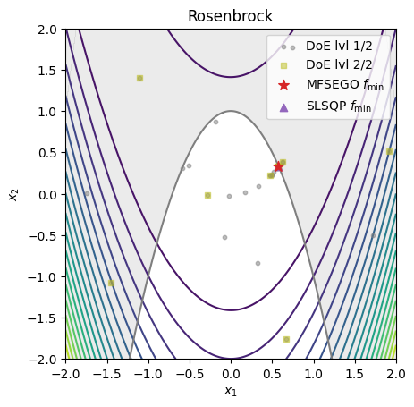
fig, ax = plt.subplots()
ax.set_title(problem.name)
ax.contour(XX, YY, Z, levels=20)
ax.contourf(XX, YY, np.where(C <= 0, np.nan, C), levels=0, colors="C7", alpha=0.15)
ax.contour(XX, YY, C, levels=[0], colors="C7")
ax.scatter(data_x[0][:, 0], data_x[0][:, 1], 10, color="C7", marker="o", alpha=0.5, label="DoE lvl 1/2", zorder=10)
ax.scatter(data_x[1][:, 0], data_x[1][:, 1], 20, color="C8", marker="s", alpha=0.5, label="DoE lvl 2/2", zorder=20)
ax.scatter(sample.x[0], sample.x[1], 75, c="C3", marker="*", label=r"MFSEGO $f_{\min}$", zorder=30)
ax.scatter(res.x[0], res.x[1], c="C4", marker="^", label=r"SLSQP $f_{\min}$", zorder=20)
ax.set_xlabel(r"$x_1$")
ax.set_ylabel(r"$x_2$")
ax.legend()
ax.set_aspect("equal")
plt.show()
best sample =
======= sample data =======
x =             [0.5776694  0.33262587]
obj =           [0.17847893]
cstr =          [1.48694119e-05]
eval_time =     [8.68021743e-07 4.98024747e-07]
------- meta data -------
iter =     19
budget =     24.5
fidelity =     1
rscv =     1.4869411850970682e-05
===========================