Multi-fidelity optimization

This page demonstrates how to minimize multi-fidelity problems. The purpose of multi-fidelity optimization is to use cheaper approximations to reduce the budget required for convergence.

This page assumes that the user is already familiar with unconstrained and constrained optimization.

import numpy as np
import matplotlib.pyplot as plt

from smt_optim import minimize

# utility method to help with plotting 2d functions
from smt_optim.utils.plot_2d import get_plot2d_data

Unconstrained multi-fidelity optimization

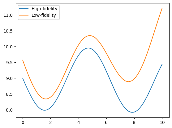
The following example illustrates how to optimize the Sasena 2002 multi-fidelity test function. The problem is defined by a high-fidelity (true) function, and a low-fidelity function which will be used as an approximation. Both functions can be expressed mathematically as:

\[\begin{split} \begin{aligned} f_{\mathrm{HF}}(x) &= -\sin(x) - \exp\!\left(\frac{x}{100}\right) + 10, \\ f_{\mathrm{LF}}(x) &= f_{\mathrm{HF}}(x) + 0.3 + 0.03\,(x - 3)^2, \\ \end{aligned} \end{split}\]

The objective will be to minimize the high-fidelity function with respect to a bounded domain. It can be expressed as:

\[ \min_{x\in \mathbb R^1} f_\text{HF}(x) \quad \text{s.t.} \quad 0 \leq x \leq 10. \]

The cell below defines the low- and high-fidelity objective functions that should be minimized.

# high-fidelity function
def sasena2002_hf(x):
    return -np.sin(x)-np.exp(x/100)+10

# low-fidelity function
def sasena2002_lf(x):
    return sasena2002_hf(x)+0.3+0.03*(x-3)**2

bounds = np.array([
    [0, 10]
])

x_valid = np.linspace(bounds[0, 0], bounds[0, 1], 101)
y_hf = sasena2002_hf(x_valid)
y_lf = sasena2002_lf(x_valid)

fig, ax = plt.subplots()
ax.plot(x_valid, y_hf, label="High-fidelity")
ax.plot(x_valid, y_lf, label="Low-fidelity")
ax.legend()
plt.show()

Starting the optimization

This example uses the minimize method to initiate the multi-fidelity Bayesian optimization. When dealing with multi-fidelity optimization, two arguments must be passed:

• objective: the function to minimize;

• design_space: the function boundary;

• costs: the sampling cost of each fidelity level.

Note

The objective argument requires a list of callables. These callables and their associated sampling costs must be ordered by level of fidelity, from lowest to highest.

Moreover, we can also pass the following optional arguments:

• max_iter: the maximum number of iterations before the program stops;

• driver_kwargs: kwargs to pass to the optimization driver. The nt_init parameter sets the number of high-fidelity samples should be in the initial DoE. In our case, nt_init is set to three samples. The seed parameter makes this example reproducible.

Note

The initial multi-fidelity DoE is generated using SMT's Nested Latin Hypercube Sampling, meaning it will have the following properties:

• Samples will be nested;
• Each lower-fidelity level will have twice as many samples as the next higher-fidelity level.

The minimize method returns a State object that contains the design of experiment (DoE) with all the low- and high-function samples. Using these samples, we can identify the best sampled function value found during the optimization process.

state = minimize(
    [sasena2002_lf, sasena2002_hf],     # in increasing order of fidelity
    bounds,
    costs=[0.2, 1.],                    # in increasing order of fidelity
    max_iter=10,
    driver_kwargs={
        "nt_init": 3,                   # number of sample in the initial Design of Experiment (DoE)
        "seed": 0,                      # makes this example reproducible
    }
)

          iter         budget           fmin           rscv       fidelity        gp_time       acq_time
             0          4.200    8.07060e+00      0.000e+00            nan            nan            nan
             1          4.400    8.07060e+00      0.000e+00              1          0.143          0.192
             2          4.600    8.07060e+00      0.000e+00              1          0.138          0.196
             3          5.800    7.98976e+00      0.000e+00              2          0.157          0.172
             4          6.000    7.98976e+00      0.000e+00              1          0.232          0.142
             5          7.200    7.91851e+00      0.000e+00              2          0.225          0.049
             6          8.400    7.91851e+00      0.000e+00              2          0.208          0.031
             7          8.600    7.91851e+00      0.000e+00              1          0.174          0.059
             8          8.800    7.91851e+00      0.000e+00              1          0.194          0.042
             9         10.000    7.91851e+00      0.000e+00              2          0.182          0.035
          iter         budget           fmin           rscv       fidelity        gp_time       acq_time
            10         11.200    7.91851e+00      0.000e+00              2          0.193          0.059

The get_best_sample class method accepts a fidelity argument that specifies the level from which to retrieve the best sample. By default, it fetches the best sample from the highest fidelity level.

print("####### Best low-fidelity sample #######")
best_sample = state.get_best_sample(fidelity=0)
print(best_sample)

print("####### Best high-fidelity sample #######")
best_sample = state.get_best_sample()
print(best_sample)

####### Best low-fidelity sample #######
======= sample data =======
x =             [1.68378806]
obj =           [8.34136876]
cstr =          []
eval_time =     [1.71440042e-05]
------- meta data -------
iter =     2
budget =     4.6000000000000005
rscv =     0.0
===========================

####### Best high-fidelity sample #######
======= sample data =======
x =             [7.88825399]
obj =           [7.91851003]
cstr =          []
eval_time =     [2.95399514e-06]
------- meta data -------
iter =     5
budget =     7.200000000000001
rscv =     0.0
===========================

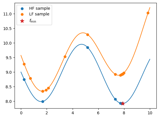
Plotting the results

The code snippet below exports all the evaluated low- and high-fidelity design points, as well as their corresponding objective values. It plots these values against their respective fidelity functions. The best sample is marked with a star.

When exporting the dataset using the export_as_dict class method, use the fidelity array to distinguish between different fidelity levels, as demonstrated below.

data = state.dataset.export_as_dict()

# retrieves the fidelity ID of each sample
fidelity = data["fidelity"]

# retrieves the low fidelity DoE
x_doe_lf = data["x"][fidelity == 0]
y_doe_lf = data["obj"][fidelity == 0]

# retrieve the high fidelity DoE
x_doe_hf = data["x"][fidelity == 1]
y_doe_hf = data["obj"][fidelity == 1]


fig, ax = plt.subplots()
# plots the HF function and samples
ax.plot(x_valid, y_hf)
ax.scatter(x_doe_hf, y_doe_hf, label="HF sample", color="C0")

# plots the LF function and samples
ax.plot(x_valid, y_lf)
ax.scatter(x_doe_lf, y_doe_lf, label="LF sample", color="C1")

# plots the best (HF) sample
ax.scatter(best_sample.x, best_sample.obj, label=r"$f_\min$", marker="*", color="C3", s=100, zorder=50)

ax.legend()
plt.show()

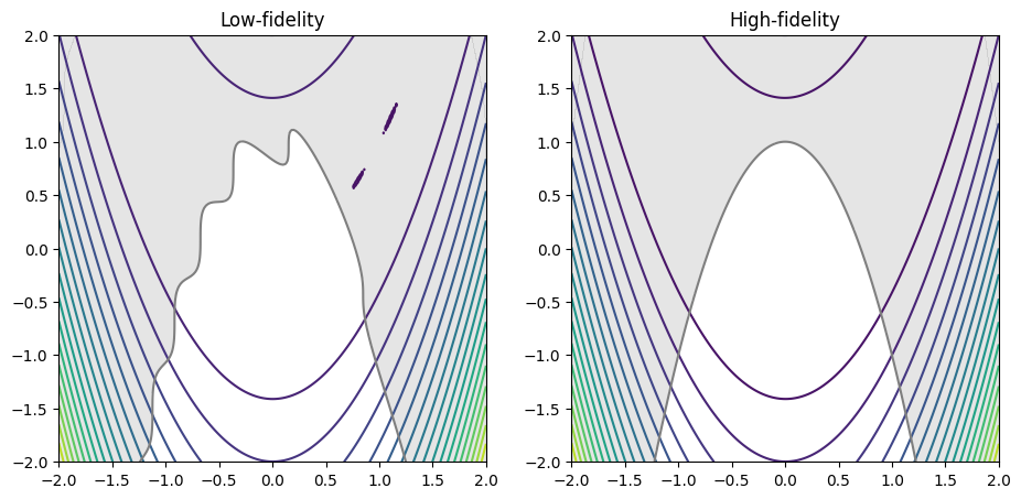
Constrained multi-fidelity optimization

The following example demonstrates how to minimize the multi-fidelity constrained Rosenbrock test problem. The high- and low fidelity objective and constraint functions are as follows:

\[\begin{split} \begin{aligned} f_{\mathrm{HF}}(x_1, x_2) &= (1 - x_1)^2 + 100\,(x_2 - x_1^2)^2, \\ f_{\mathrm{LF}}(x_1, x_2) &= f_{\mathrm{HF}}(x_1, x_2) + 0.1\,\sin(10x_1 + 5x_2), \\ g_{\mathrm{HF}}(x_1, x_2) &= x_1^2 + \sqrt{x_2 - 1}, \\ g_{\mathrm{LF}}(x_1, x_2) &= g_{\mathrm{HF}}(x_1, x_2) - 0.1\,\sin(10x_1 + 5x_2). \end{aligned} \end{split}\]

The objective will be to minimize the high fidelity objective function with respect to the high-fidelity inequality constraint:

\[\begin{split} \begin{aligned} \min_{x\in \mathbb R^2} \quad & f_\text{HF}(\boldsymbol x) \\ \text{s.t.} \quad & -2 \leq x_i \leq 2 \quad i = 1, 2 \\ & g_\text{HF} (\boldsymbol x) \leq 0. \end{aligned} \end{split}\]

The cell below defines the low- and high-fidelity objective and constraint function.

Note

The minimize method requires all quantities of interest (QoI) (e.g.: objectives and constraints) to have the same number of fidelities.

# defines the high-fidelity objective function
def rosenbrock_hf(x):
    return (1 - x[0])**2 + 100*(x[1] - x[0]**2)**2

# defines the low-fidelity objective function
def rosenbrock_lf(x):
    return rosenbrock_hf(x) + 0.1*np.sin(10*x[0] + 5*x[1])

# defines the high-fidelity constraint function
def constraint_hf(x):
    return -(-x[0]**2 - (x[1] - 1)**1/2)

# defines the low-fidelity constraint function
def constraint_lf(x):
    return constraint_hf(x) - 0.1*np.sin(10*x[0] + 5*x[1])

# defines the problem boundary
bounds = np.array([
    [-2, 2],
    [-2, 2]
])

# plots the low- and high-fidelity test problem
XX, YY, Z_hf = get_plot2d_data(rosenbrock_hf, bounds, 201)
_, _, Z_lf = get_plot2d_data(rosenbrock_lf, bounds, 201)
_, _, G_hf = get_plot2d_data(constraint_hf, bounds, 201)
_, _, G_lf = get_plot2d_data(constraint_lf, bounds, 201)

fig, ax = plt.subplots(1, 2, figsize=(11, 7))
ax[0].set_title("Low-fidelity")
ax[0].contour(XX, YY, Z_lf, levels=20)
ax[0].contourf(XX, YY, np.where(G_lf <= 0, np.nan, G_lf), levels=0, colors="C7", alpha=0.20)
ax[0].contour(XX, YY, G_lf, levels=[0], colors="C7")
ax[0].set_aspect("equal")

ax[1].set_title("High-fidelity")
ax[1].contour(XX, YY, Z_hf, levels=20)
ax[1].contourf(XX, YY, np.where(G_hf <= 0, np.nan, G_hf), levels=0, colors="C7", alpha=0.20)
ax[1].contour(XX, YY, G_hf, levels=[0], colors="C7")
ax[1].set_aspect("equal")

plt.show()

Starting the optimization

The minimize method is called to begin the constrained multi-fidelity Bayesian optimization. Three arguments must be passed when dealing with constrained multi-fidelity optimization:

• objective: the function to minimize;

• design_space: the function boundary;

• costs: the sampling cost of each fidelity level;

• constraints: the constraint definitions.

Note

The objective and the constraints callables, as well as the sampling costs must be ordered in increasing level of fidelity and must have the identical number of callables.

Moreover, we can also pass the following optional arguments:

• max_iter: the maximum number of iterations before the program stops;

• max_budget: the maximum budget before the program stops. The budget is computed with the sampling costs;

• driver_kwargs: kwargs to pass to the optimization driver. The seed parameter makes this example reproducible;

• strategy_kwargs: kwargs to pass to the acquisition strategy.

Note

The strategy_kwargs depend on the AcquisitionStrategy selected by the minimize method. For a multi-fidelity problem (constrained or unconstrained), the MFSEGO acquisition strategy is selected. The valid arguments can be consulted via the API reference.

The minimize method returns a State object that contains the design of experiment (DoE) with all the low- and high-function samples. Using these samples, we can identify the best sampled function value found during the optimization process.

# defines the inequality constraint
constraint = [
    {
        "fun": [constraint_lf, constraint_hf],      # in increasing order of fidelity
        "upper": 0.,                                # equivalent to: g(x) <= 0
    }
]

state = minimize(
    [rosenbrock_lf, rosenbrock_hf],                 # in increasing order of fidelity
    bounds,
    costs=[0.2, 1.],
    constraints=constraint,
    max_iter=30,
    max_budget=15.,
    # arguments passed to the optimization driver
    driver_kwargs={
        "seed": 0
    },
    # arguments passed to the acquisition strategy
    strategy_kwargs={
        "fidelity_crit": "pessimistic",
        "sp_method": "Cobyla",
        "sp_tol": 1e-4
    }
)

          iter         budget           fmin           rscv       fidelity        gp_time       acq_time
             0          7.000    2.64887e+00      0.000e+00            nan            nan            nan
             1          7.200    2.64887e+00      0.000e+00              1          0.846          1.766
             2          7.400    2.64887e+00      0.000e+00              1          0.938          2.028
             3          7.600    2.64887e+00      0.000e+00              1          0.997          1.535
             4          7.800    2.64887e+00      0.000e+00              1          1.001          1.693
             5          8.000    2.64887e+00      0.000e+00              1          0.766          1.723
             6          8.200    2.64887e+00      0.000e+00              1          0.834          1.769
             7          8.400    2.64887e+00      0.000e+00              1          0.747          2.083
             8          9.600    2.64887e+00      0.000e+00              2          0.781          1.766
             9          9.800    2.64887e+00      0.000e+00              1          0.822          1.042
          iter         budget           fmin           rscv       fidelity        gp_time       acq_time
            10         10.000    2.64887e+00      0.000e+00              1          1.181          1.307
            11         10.200    2.64887e+00      0.000e+00              1          0.937          1.855
            12         10.400    2.64887e+00      0.000e+00              1          0.722          1.100
            13         11.600    2.63493e-01      0.000e+00              2          0.941          1.013
            14         11.800    2.63493e-01      0.000e+00              1          0.883          1.402
            15         13.000    1.93389e-01      0.000e+00              2          0.751          1.260
            16         14.200    1.78495e-01      3.382e-05              2          0.691          1.084
            17         14.400    1.78495e-01      3.382e-05              1          0.796          0.951
            18         14.600    1.78495e-01      3.382e-05              1          0.651          1.142
            19         14.800    1.78495e-01      3.382e-05              1          0.615          1.015
          iter         budget           fmin           rscv       fidelity        gp_time       acq_time
            20         16.000    1.78495e-01      3.382e-05              2          0.804          1.064

Plotting the results

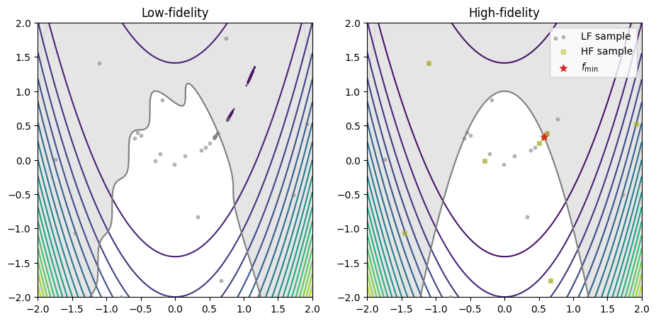
The code snippet below exports all the evaluated low- and high-fidelity design points, as well as their corresponding objective values, plotting them against their respective fidelity function. The best sample is marked with a star.

When exporting the dataset using the export_as_dict class method, use the fidelity array to distinguish between different fidelity levels, as demonstrated below.

# gets the best sample (minimum feasible objective value)
best_sample = state.get_best_sample()

data = state.dataset.export_as_dict()

# retrieves the fidelity ID of each sample
fidelity = data["fidelity"].ravel()

# retrieves the low fidelity DoE
x_doe_lf = data["x"][fidelity == 0, :]
# y_doe_lf = data["obj"][fidelity == 0]

# retrieve the high fidelity DoE
x_doe_hf = data["x"][fidelity == 1, :]
# y_doe_hf = data["obj"][fidelity == 1]

fig, ax = plt.subplots(1, 2, figsize=(11, 7))
ax[0].set_title("Low-fidelity")
ax[0].contour(XX, YY, Z_lf, levels=20)
ax[0].contourf(XX, YY, np.where(G_lf <= 0, np.nan, G_lf), levels=0, colors="C7", alpha=0.2)
ax[0].contour(XX, YY, G_lf, levels=[0], colors="C7")
ax[0].set_aspect("equal")

ax[0].scatter(x_doe_lf[:, 0], x_doe_lf[:, 1], s=10, color="C7", alpha=0.5, label="LF sample", zorder=50)

ax[1].set_title("High-fidelity")
ax[1].contour(XX, YY, Z_hf, levels=20)
ax[1].contourf(XX, YY, np.where(G_hf <= 0, np.nan, G_hf), levels=0, colors="C7", alpha=0.2)
ax[1].contour(XX, YY, G_hf, levels=[0], colors="C7")
ax[1].set_aspect("equal")

# scatters the LF samples
ax[1].scatter(x_doe_lf[:, 0], x_doe_lf[:, 1], s=10, color="C7", alpha=0.5, label="LF sample", zorder=50)
# scatters the HF samples
ax[1].scatter(x_doe_hf[:, 0], x_doe_hf[:, 1], s=20, color="C8", alpha=0.5, marker="s", label="HF sample", zorder=60)
# plots the best sample
ax[1].scatter(best_sample.x[0], best_sample.x[1], s=50, color="C3", marker="*", label=r"$f_\min$", zorder=100)

ax[1].legend(loc="upper right")
plt.show()

Many multi-fidelity levels optimization

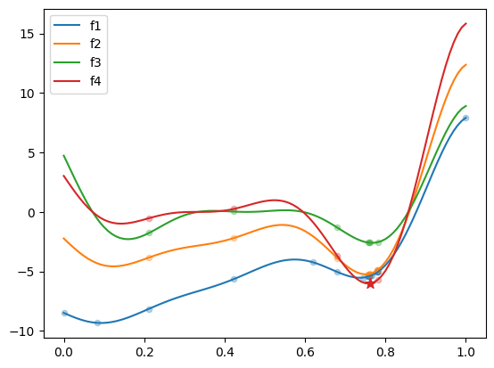
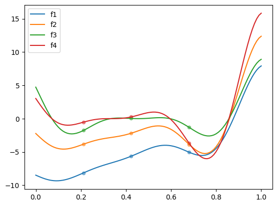
The following example demonstrates how to minimize the Forrester multi-fidelity test problem with 4 fidelity levels. The nt_init parameter corresponds to the number of high-fidelity samples in initial DOE. By default, each lower level has twice as many samples. Here, we propose to start the optimization with a predefined nested DOE, where each level has 3 samples.

The 4 fidelity levels are defined by:

\[\begin{split} \begin{aligned} f_{\mathrm{4}}(x) &= (6x - 2)^2 \sin(12x-4), \\ f_{\mathrm{3}}(x) &= (5.5x - 2.5)^2 \sin(12x - 4), \\ f_{\mathrm{2}}(x) &= 0.75 f_{\mathrm{4}}(x) + 5(x - 0.5) - 2, \\ f_{\mathrm{1}}(x) &= 0.5 f_{\mathrm{4}}(x) + 10(x - 0.5) - 5. \end{aligned} \end{split}\]

The objective is to minimize the highest fidelity level:

\[\begin{split} \begin{aligned} \min_{x\in \mathbb R^1} \quad & f_\text{4}(x) \\ \text{s.t.} \quad & 0 \leq x \leq 1\\ \end{aligned} \end{split}\]

The get_problem method is used to import the test problem, and SMT’s LHS sampler is used to generate the initial DOE. The figure below plots the 4 fidelity levels, along with the corresponding initial nested DOE.

from smt_optim.benchmarks.registry import get_problem
from smt.sampling_methods import LHS

# fetch the Forrester test problem
problem = get_problem("Forrester")

# create custom nested DOE, where each level has the same number of samples
sampler = LHS(xlimits=problem.bounds, criterion="ese", seed=0)
doe_hf = sampler(3)
doe = [doe_hf for _ in range(problem.num_fidelity)]

x_valid = np.linspace(problem.bounds[0, 0], problem.bounds[0, 1], 101)

fig, ax = plt.subplots()
for lvl in range(problem.num_fidelity):
    ax.scatter(doe[lvl], problem.objective[lvl](doe[lvl]), 20, alpha=0.5)
    ax.plot(x_valid, problem.objective[lvl](x_valid), label=f"f{lvl+1}")

ax.legend()
plt.show()

Starting the optimization

The optimization is started by calling the minimize method. The custom DOE is provided to the xt_init driver keyword argument. It should be noted that the costs parameter expects 4 costs to be provided, one for each level.

state = minimize(
    problem.objective,
    problem.bounds,
    costs=[1/1000, 1/100, 1/10, 1.],
    max_iter=15,
    max_budget=10.,
    # arguments passed to the optimization driver
    driver_kwargs={
        "xt_init": doe,
        "seed": 0,
    },
    strategy_kwargs={
        "var_red_corr": "max",  # more numerically stable with many fidelity levels
    }
)

          iter         budget           fmin           rscv       fidelity        gp_time       acq_time
             0          3.333   -3.69868e+00      0.000e+00            nan            nan            nan
             1          3.334   -3.69868e+00      0.000e+00              1          0.189          0.200
             2          3.335   -3.69868e+00      0.000e+00              1          0.230          0.307
             3          3.336   -3.69868e+00      0.000e+00              1          0.212          0.465
             4          3.337   -3.69868e+00      0.000e+00              1          0.215          0.483
             5          3.338   -3.69868e+00      0.000e+00              1          0.289          0.674
             6          3.339   -3.69868e+00      0.000e+00              1          0.267          0.451
             7          3.350   -3.69868e+00      0.000e+00              2          0.232          0.395
             8          3.461   -3.69868e+00      0.000e+00              3          0.269          0.498
             9          3.572   -3.69868e+00      0.000e+00              3          0.283          0.455
          iter         budget           fmin           rscv       fidelity        gp_time       acq_time
            10          3.573   -3.69868e+00      0.000e+00              1          0.352          0.535
            11          3.584   -3.69868e+00      0.000e+00              2          0.312          0.568
            12          3.595   -3.69868e+00      0.000e+00              2          0.358          0.780
            13          4.706   -5.70783e+00      0.000e+00              4          0.332          0.495
            14          5.817   -6.01300e+00      0.000e+00              4          0.371          0.417
            15          5.818   -6.01300e+00      0.000e+00              1          0.376          0.349

Plotting the results

The code snippet below exports all the evaluated design points, as well as their corresponding objective values, plotting them against their respective fidelity function. The best sample is marked with a star.

# fetch best sample
best_sample = state.get_best_sample()

data = state.dataset.export_as_dict()

fig, ax = plt.subplots()
for lvl in range(problem.num_fidelity):

    x = data["x"].ravel()
    obj = data["obj"].ravel()
    fid_mask = data["fidelity"].ravel() == lvl
    ax.scatter(x[fid_mask], obj[fid_mask], 20, alpha=0.3)

    ax.plot(x_valid, problem.objective[lvl](x_valid), label=f"f{lvl+1}")

ax.scatter(best_sample.x[0], best_sample.obj[0], 75, color="C3", marker="*")

ax.legend()
plt.show()