Unconstrained optimization - EGO#
import numpy as np
from matplotlib import pyplot as plt

from smt_optim.benchmarks.registry import get_problem

from smt_optim.core import Driver, ObjectiveConfig, ConstraintConfig, DriverConfig, Problem

from smt_optim.surrogate_models.smt import SmtAutoModel, SmtGPX

from smt_optim.acquisition_strategies import MFSEGO
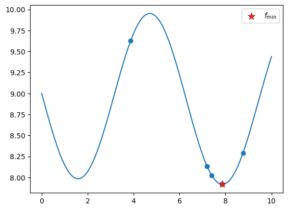
Unconstrained 1D optimization#
This example will use the Sasena test function (2002). The bounds are \([0, 10]\)
def sasena_2002(x: np.ndarray):
    return -np.sin(x) - np.exp(x / 100) + 10

bounds = np.array([[0, 10]])
obj_config = ObjectiveConfig(
    objective=[sasena_2002],
    type="minimize",
    surrogate=SmtGPX,           # set which GP to model the objective
)

prob_definition = Problem(
    obj_configs=[obj_config],
    design_space=bounds,
)
Once the problem is initialized, we can configure the optimization driver. We can set the configuration using the DriverConfig dataclass and then initialize the driver with the Driver class.
In our example, we set the following parameters:
max_itercorresponds to the maximum number of iteration that will be performed.nt_initcorresponds to the number of samples in the initial DOE. The initial DOE will be generated using LHS.verbosecan be set toTrueorFalse. If set toTruesome basic information will be printed at the end of each iteration.seedallows to reproduce optimization run.
The MFSEGO optimization strategy must be pass to perform EGO (unconstrained optimization), SEGO (constrained optimization) and MFSEGO (unconstrained or constrained and multi-fidelity optimization).
driver_config = DriverConfig(
    max_iter = 5,              # stopping criterion
    nt_init = 2,                # number of sample in the initial DoE
    verbose = True,
    seed=42,
)

# configure the optimizer. Note: if a single fidelity level is given to the MFSEGO acquisition strategy, it falls back to the SEGO framework.
driver = Driver(prob_definition, driver_config, MFSEGO)
We can launch the optimization using the optimize() class method. It will return a State object.
# return the optimization data
state = driver.optimize()
          iter         budget           fmin           rscv       fidelity        gp_time       acq_time
             1              3    8.13516e+00      0.000e+00              1          0.013          0.016
             2              4    8.02643e+00      0.000e+00              1          0.011          0.036
             3              5    8.02643e+00      0.000e+00              1          0.016          0.030
             4              6    7.91867e+00      0.000e+00              1          0.016          0.029
             5              7    7.91829e+00      0.000e+00              1          0.016          0.025
Once the optimization terminated, we can recover the best sample using the get_best_sample() class method. It will return a Sample dataclass with the lowest objective value.
sample = state.get_best_sample()
sample
======= sample data =======
x =             [7.85449065]
obj =           [7.9182882]
cstr =          []
eval_time =     [6.25301618e-06]
------- meta data -------
iter =     5
budget =     7
fidelity =     0
rscv =     0.0
===========================
We can only also recover the entire DOE using the dataset attribute.
dataset = state.dataset

data = dataset.export_as_dict()
xt = data["x"]
yt = data["obj"]
x_test = np.linspace(0, 10, 201)
y_test = sasena_2002(x_test)

fig, ax = plt.subplots()
ax.plot(x_test, y_test)
ax.scatter(xt, yt)
ax.scatter(sample.x, sample.obj, 100, marker="*", color="C3", zorder=20, label=r"$f_\min$")

ax.legend()
plt.show()
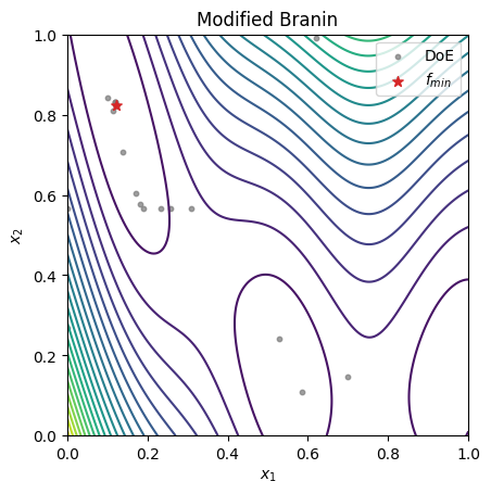
Unconstrained 2D optimization#
def modified_branin(x):
    """
    Engineering Design via Surrogate Modelling: A Practical Guide
    A. I. J. Forrester, A. Sóbester and A. J. Keane
    2008
    """
    X1 = 15 * x[0] - 5
    X2 = 15 * x[1]

    a = 1
    b = 5.1 / (4 * np.pi ** 2)
    c = 5 / np.pi
    d = 6
    e = 10
    ff = 1 / (8 * np.pi)
    f = (a * (X2 - b * X1 ** 2 + c * X1 - d) ** 2 + e * (1 - ff) * np.cos(X1) + e) + 5 * x[0]

    return f


bounds = np.array([
    [0, 1],
    [0, 1],
])
obj_config = ObjectiveConfig(
    [modified_branin],
    type="minimize",
    surrogate=SmtGPX,
)

prob_definition = Problem(
    obj_configs=[obj_config],
    design_space=bounds,            # problem bounds
)

opt_config = DriverConfig(
    max_iter = 20,
    nt_init = 3,
    verbose = True,
    scaling = True,
    seed=42,
)

driver = Driver(prob_definition, opt_config, MFSEGO)

state = driver.optimize()
          iter         budget           fmin           rscv       fidelity        gp_time       acq_time
             1              4    1.56584e+01      0.000e+00              1          0.013          0.049
             2              5    1.56584e+01      0.000e+00              1          0.018          0.060
             3              6    1.56584e+01      0.000e+00              1          0.018          0.044
             4              7    1.20846e+01      0.000e+00              1          0.019          0.077
             5              8    8.01942e+00      0.000e+00              1          0.025          0.052
             6              9    7.30910e+00      0.000e+00              1          0.023          0.076
             7             10    5.99029e+00      0.000e+00              1          0.024          0.062
             8             11    4.66766e+00      0.000e+00              1          0.021          0.091
             9             12    2.68915e+00      0.000e+00              1          0.022          0.063
            10             13    1.74179e+00      0.000e+00              1          0.022          0.070
          iter         budget           fmin           rscv       fidelity        gp_time       acq_time
            11             14    1.29634e+00      0.000e+00              1          0.026          0.076
            12             15    1.29634e+00      0.000e+00              1          0.036          0.077
            13             16    1.01964e+00      0.000e+00              1          0.037          0.123
            14             17    1.01832e+00      0.000e+00              1          0.030          0.074
            15             18    1.01692e+00      0.000e+00              1          0.035          0.099
            16             19    1.01159e+00      0.000e+00              1          0.033          0.088
            17             20    1.01159e+00      0.000e+00              1          0.039          0.134
            18             21    1.01157e+00      0.000e+00              1          0.031          0.092
            19             22    1.01157e+00      0.000e+00              1          0.030          0.129
            20             23    1.01157e+00      0.000e+00              1          0.033          0.120
# get the best sample in the dataset
sample = state.get_best_sample()
xt = state.dataset.export_as_dict()["x"]

X = np.linspace(bounds[0, 0], bounds[0, 1], 201)
Y = np.linspace(bounds[1, 0], bounds[1, 1], 201)
XX, YY = np.meshgrid(X, Y)

data = np.vstack((XX.ravel(), YY.ravel())).T
z = np.empty(data.shape[0])

for i in range(data.shape[0]):
    z[i] = modified_branin(data[i, :])

Z = z.reshape(XX.shape)

fig, ax = plt.subplots()

ax.set_title("Modified Branin")

# plot the test function
ax.contour(XX, YY, Z, levels=20)

# plot the points in the final DoE
ax.scatter(xt[:, 0], xt[:, 1], 10, color="C7", alpha=0.75, label="DoE")

# plot the best sample in the final DoE
ax.scatter(sample.x[0], sample.x[1], 50, c="C3", marker="*", label=r"$f_{min}$", zorder=30)

ax.set_xlabel(r"$x_1$")
ax.set_ylabel(r"$x_2$")

ax.legend()
ax.set_aspect("equal")
plt.show()