
Multi-objective optimization#
This notebook demonstrates how to perform multi-objective Bayesian optimization using the MO-SEGO (Multi-Objective Super Efficient Global Optimization) framework. Constrained and multi-fidelity optimization are also supported in the multi-objective framework.
In multi-objective optimization, we are interested in minimizing multiple \(n\) objectives with respect to constraints \(\boldsymbol{g}\) and \(\boldsymbol{h}\) (if applicable).
import numpy as np
import matplotlib.pyplot as plt

from smt_optim.core import Driver, ObjectiveConfig, ConstraintConfig, DriverConfig, Problem

from smt_optim.surrogate_models.smt import SmtGPX,SmtAutoModel

from smt_optim.acquisition_strategies.mosego import MOSEGO
from smt_optim.acquisition_functions import init_ehvi_2o, init_mpi
from smt_optim.utils.multi_obj import get_pf_from_dataset

from smt_optim.benchmarks.registry import get_problem

from smt_optim.utils.multi_obj import PymooStateWrapper
from smt_optim.benchmarks.base import PymooWrapper
from pymoo.algorithms.moo.nsga2 import NSGA2
from pymoo.optimize import minimize
Multi-objective optimization#
The following example illustrates how to find the ZDT1’s Pareto front using the MO-SEGO framework. The code cell below imports the test problem using the get_problem method and plots both objective. The ZDT1 is defined as follows:
where \(d=2\) is the number of variables, \(g(\boldsymbol x) = 1 + \frac{9}{d - 1}\sum_{i=2}^{d}x_i\), and \(h(f_1, \; g) = 1 - \sqrt{f_1/g}\).
problem = get_problem("ZDT1")
problem.set_dim(2)
Starting the optimization#
The code cell shows how to initialize both objectives, the problem configuration, and the driver configuration. The driver is initialized with the MOSEGO acquisition strategy, which is designed for multiple objective optimization. The Expected Hypervolume Improved (EHVI) acquisition function is used in this example.
# initialize the first objective configuration
obj1_config = ObjectiveConfig(
    [problem.f1],
    type="minimize",
    surrogate=SmtGPX,
)

# initialize the second objective configuration
obj2_config = ObjectiveConfig(
    [problem.f2],
    type="minimize",
    surrogate=SmtGPX,
)

# initialize the problem configuration
prob_definition = Problem(
    obj_configs=[obj1_config, obj2_config],
    design_space=problem.bounds,
)

nt_init = 5

# initialize the driver
opt_config = DriverConfig(
    max_iter = 20,
    nt_init = nt_init,
    verbose = True,
    scaling = True,
    seed=0,
)

driver = Driver(prob_definition, opt_config, MOSEGO, strategy_kwargs={"acq_init": init_ehvi_2o,})

# starts the optimization process
state = driver.optimize()
          iter         budget             HV        spacing       fidelity        gp_time       acq_time
             0              5    4.19380e+00    1.51008e+00            nan            nan            nan
             1              6    6.03242e+00    0.00000e+00              1          0.007          0.664
             2              7    6.25988e+00    0.00000e+00              1          0.006          1.065
             3              8    6.31523e+00    3.19955e-01              1          0.007          0.791
             4              9    6.39097e+00    9.42216e-02              1          0.006          0.725
             5             10    6.40817e+00    1.16361e-01              1          0.006          0.664
             6             11    6.43248e+00    6.33432e-02              1          0.006          0.688
             7             12    6.44221e+00    6.19025e-02              1          0.007          0.741
             8             13    6.44999e+00    4.17557e-02              1          0.007          0.435
             9             14    6.44999e+00    4.17557e-02              1          0.008          0.683
          iter         budget             HV        spacing       fidelity        gp_time       acq_time
            10             15    6.44999e+00    4.17557e-02              1          0.008          0.438
            11             16    6.45317e+00    2.35243e-02              1          0.008          0.444
            12             17    6.45317e+00    2.35243e-02              1          0.007          0.349
            13             18    6.45317e+00    2.35243e-02              1          0.008          0.347
            14             19    6.45317e+00    2.35243e-02              1          0.006          0.318
            15             20    6.45317e+00    2.35243e-02              1          0.008          0.334
            16             21    6.45317e+00    2.35243e-02              1          0.009          0.330
            17             22    6.45317e+00    2.35243e-02              1          0.009          0.305
            18             23    6.45317e+00    2.35243e-02              1          0.008          0.314
            19             24    6.45317e+00    2.35243e-02              1          0.009          0.457
          iter         budget             HV        spacing       fidelity        gp_time       acq_time
            20             25    6.45317e+00    2.35243e-02              1          0.009          0.319
Plotting the results#
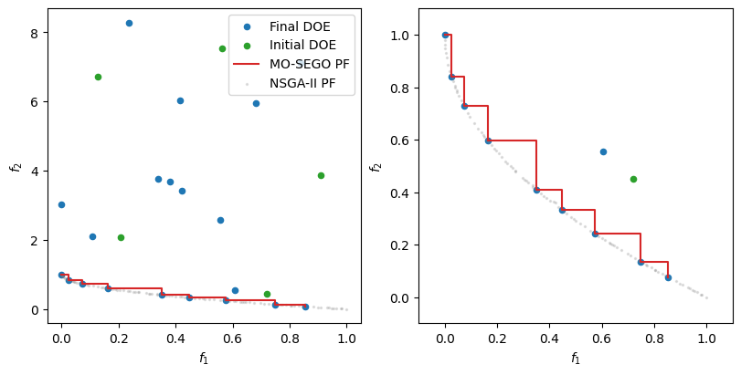
The code cell below extracts the Pareto front (PF) from the final DOE using the get_pf_from_dataset method. The figure shows the final DOE, the initial DOE, and compares the Pareto front obtained with MO-SEGO with one obtained with Pymoo’s NSGA-II algorithm.
# ======= MO-SEGO Pareto Front =======
data = driver.state.dataset.export_as_dict()
obj = data["obj"]

obj_par = get_pf_from_dataset(state.dataset)
sorted_idx = np.argsort(obj_par[:, 0])
obj_par = obj_par[sorted_idx, :]

# ======= NSGA-II Pareto Front =======
pymoo_problem = PymooWrapper(problem)

# find the Pareto front with Pymoo's NSGA-II implementation
algorithm = NSGA2(pop_size=100, seed=0)
pymoo_res = minimize(pymoo_problem, algorithm, ("n_gen", 100), seed=0)

# ======= Plot optimization and solution pareto front =======
fig, ax = plt.subplots(1, 2, layout="constrained", figsize=(8, 4))

for i in range(2):
    ax[i].scatter(obj[nt_init:, 0], obj[nt_init:, 1], 20, color="C0", label="Final DOE")
    ax[i].scatter(obj[:nt_init, 0], obj[:nt_init, 1], 20, color="C2", label="Initial DOE")

    # PF obtained through optimization
    ax[i].step(obj_par[:, 0], obj_par[:, 1], where="post", color="C3", zorder=20, label="MO-SEGO PF")

    # NSGA-II PF
    ax[i].scatter(pymoo_res.F[:, 0], pymoo_res.F[:, 1], 2, color="C7", alpha=0.2, zorder=10, label="NSGA-II PF")

    ax[i].set_xlabel(r"$f_1$")
    ax[i].set_ylabel(r"$f_2$")

ax[1].set_xlim((-0.1, 1.1))
ax[1].set_ylim((-0.1, 1.1))
ax[0].legend()
plt.show()
Constrained multi-objective optimization#
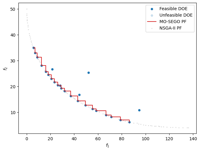
The following example illustrates how to find the Pareto front when subjected to constraints. The get_problem method is used to import the BNH test problem, which is defined as follows:
problem = get_problem("BNH")
obj1_config = ObjectiveConfig(
    [problem.objective[0]],
    type="minimize",
    surrogate=SmtGPX,
)

obj2_config = ObjectiveConfig(
    [problem.objective[1]],
    type="minimize",
    surrogate=SmtGPX,
)

cstr1_config = ConstraintConfig(
    [problem.constraints[0]],
    upper=0.,
    surrogate=SmtGPX,
)

cstr2_config = ConstraintConfig(
    [problem.constraints[1]],
    upper=0.,
    surrogate=SmtGPX,
)

prob_definition = Problem(
    obj_configs=[obj1_config, obj2_config],
    cstr_configs=[cstr1_config, cstr2_config],
    design_space=problem.bounds,            # problem bounds
)

nt_init = 5

opt_config = DriverConfig(
    max_iter = 20,
    nt_init = nt_init,
    verbose = True,
    scaling = True,
    seed=0,
)

driver = Driver(prob_definition, opt_config, MOSEGO, strategy_kwargs={"relax_constraints": 2.0})

state = driver.optimize()
          iter         budget             HV        spacing       fidelity        gp_time       acq_time
             0              5    1.12241e+03    3.97964e+00            nan            nan            nan
             1              6    1.32685e+03    3.61912e+00              1          0.022          2.638
             2              7    1.42749e+03    7.44827e+00              1          0.024          3.090
             3              8    1.49854e+03    6.20135e+00              1          0.033          3.053
             4              9    1.56097e+03    4.15355e+00              1          0.026          2.555
             5             10    1.59283e+03    3.68272e+00              1          0.025          2.857
             6             11    1.62403e+03    1.86295e+00              1          0.029          4.199
             7             12    1.65328e+03    1.94350e+00              1          0.033          4.309
             8             13    1.67065e+03    1.76778e+00              1          0.028          4.950
             9             14    1.68458e+03    2.54511e+00              1          0.032          5.707
          iter         budget             HV        spacing       fidelity        gp_time       acq_time
            10             15    1.69633e+03    2.22168e+00              1          0.032          4.757
            11             16    1.70742e+03    2.34999e+00              1          0.033          4.522
            12             17    1.71855e+03    2.35756e+00              1          0.034          3.948
            13             18    1.72586e+03    1.36704e+00              1          0.032          5.137
            14             19    1.73167e+03    2.19324e+00              1          0.035          4.820
            15             20    1.73617e+03    2.11912e+00              1          0.033          3.730
            16             21    1.74186e+03    1.85392e+00              1          0.037          4.508
            17             22    1.74514e+03    1.96599e+00              1          0.037          2.966
            18             23    1.74872e+03    1.94667e+00              1          0.035          3.375
            19             24    1.75214e+03    1.96990e+00              1          0.036          2.882
          iter         budget             HV        spacing       fidelity        gp_time       acq_time
            20             25    1.75550e+03    2.06845e+00              1          0.039          2.982
Plotting the results#
# ======= MO-SEGO Pareto Front =======
data = driver.state.dataset.export_as_dict()
obj = data["obj"]
feas_mask = data["rscv"] <= 1e-4

obj_par = get_pf_from_dataset(state.dataset)
sorted_idx = np.argsort(obj_par[:, 0])
obj_par = obj_par[sorted_idx, :]

# ======= NSGA-II Pareto Front =======
pymoo_problem = PymooWrapper(problem)

# find the Pareto front with Pymoo's NSGA-II implementation
algorithm = NSGA2(pop_size=100, seed=0)
pymoo_res = minimize(pymoo_problem, algorithm, ("n_gen", 100), seed=0)

# ======= Plot optimization and solution pareto front =======
fig, ax = plt.subplots(layout="constrained")

ax.scatter(obj[feas_mask, 0], obj[feas_mask, 1], 20, color="C0", label="Feasible DOE")
ax.scatter(obj[~feas_mask, 0], obj[~feas_mask, 1], 20, color="C0", alpha=0.2, label="Unfeasible DOE")

# PF obtained through optimization
ax.step(obj_par[:, 0], obj_par[:, 1], where="post", color="C3", zorder=20, label="MO-SEGO PF")

# Solution PF
ax.scatter(pymoo_res.F[:, 0], pymoo_res.F[:, 1], 2, color="C7", alpha=0.2, zorder=10, label="NSGA-II PF")

ax.set_xlabel(r"$f_1$")
ax.set_ylabel(r"$f_2$")

ax.legend()
plt.show()
Applying NSGA-II (Pymoo) on the surrogate models#
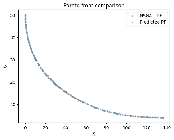
Users can use the PymooStateWrapper to convert a state object into a Pymoo Problem object. Below, the NSGA-II algorithm is applied on the objective and constraint models to find a predicted Pareto front.
# Create a pymoo problem object from the SMT-Optim state object
pymoo_state = PymooStateWrapper(state)

algorithm = NSGA2(pop_size=100, seed=1)
state_res = minimize(pymoo_problem, algorithm, ("n_gen", 100), seed=1)

fig, ax = plt.subplots()

ax.scatter(pymoo_res.F[:, 0], pymoo_res.F[:, 1], 10, color="C7", alpha=0.5, zorder=10, label="NSGA-II PF")

ax.scatter(state_res.F[:, 0], state_res.F[:, 1], 10, color="C0", alpha=0.5, label="Predicted PF")

ax.legend()
ax.set_title("Pareto front comparison")
ax.set_xlabel(r"$f_1$")
ax.set_ylabel(r"$f_2$")
plt.show()
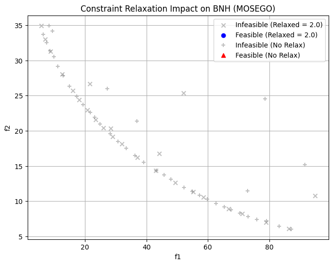
Effect of Constraint Relaxation#
Let’s compare the previous MOSEGO run (with relax_constraints=2.0) against a run with no relaxation (relax_constraints=0.0).
Without relaxation, the optimizer uses the strict surrogate model mean for constraints, which can lead to it being overly conservative or getting stuck if the initial surrogate model is poorly calibrated near the boundaries.
opt_config_no_relax = DriverConfig(
    max_iter=30,
    nt_init=10,
    seed=0,
)

driver_no_relax = Driver(prob_definition, opt_config_no_relax, MOSEGO, strategy_kwargs={"relax_constraints": 0.0})
state_no_relax = driver_no_relax.optimize()
plt.figure(figsize=(8, 6))

y_evaluated = np.array(state.dataset.export_as_dict()["obj"])
c_evaluated = np.array(state.dataset.export_as_dict()["cstr"])
feasible = (c_evaluated[:, 0] <= 1.0) & (c_evaluated[:, 1] >= 0.0)

y_evaluated_no_relax = np.array(state_no_relax.dataset.export_as_dict()["obj"])
c_evaluated_no_relax = np.array(state_no_relax.dataset.export_as_dict()["cstr"])
feasible_no_relax = (c_evaluated_no_relax[:, 0] <= 1.0) & (c_evaluated_no_relax[:, 1] >= 0.0)

plt.scatter(y_evaluated[~feasible, 0], y_evaluated[~feasible, 1], c='gray', marker='x', alpha=0.5, label='Infeasible (Relaxed = 2.0)')
plt.scatter(y_evaluated[feasible, 0], y_evaluated[feasible, 1], c='blue', marker='o', label='Feasible (Relaxed = 2.0)')

plt.scatter(y_evaluated_no_relax[~feasible_no_relax, 0], y_evaluated_no_relax[~feasible_no_relax, 1], c='gray', marker='+', alpha=0.5, label='Infeasible (No Relax)')
plt.scatter(y_evaluated_no_relax[feasible_no_relax, 0], y_evaluated_no_relax[feasible_no_relax, 1], c='red', marker='^', label='Feasible (No Relax)')

plt.xlabel('f1')
plt.ylabel('f2')
plt.legend()
plt.title('Constraint Relaxation Impact on BNH (MOSEGO)')
plt.grid(True)
plt.show()
Constrained, multi-fidelity, and multi-objective optimization#
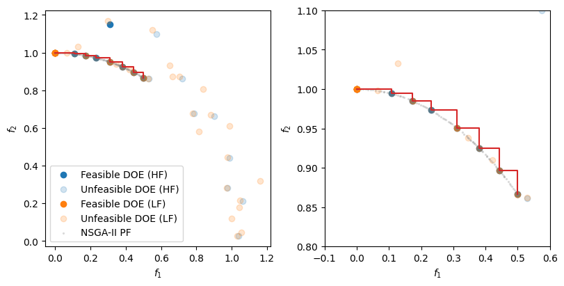
The following example demonstrates how to find the Pareto front of a constrained multi-objective problem, for which low-fidelity approximations exist.
This example uses the DTLZ5 test function which has 2 fidelity levels and 1 constraint.
The code cell below imports the DTLZ5 test function, initializes the objectives, the constraint, the problem configuration, and the driver configuration, and starts the optimization process.
Starting the optimization#
problem = get_problem("DTLZ5")
problem.set_dim(4)

obj_config = ObjectiveConfig(
    problem.objective[0],
    type="minimize",
    surrogate=SmtAutoModel,
)

obj_config2 = ObjectiveConfig(
    problem.objective[1],
    type="minimize",
    surrogate=SmtAutoModel,
)

cstr_config = ConstraintConfig(
    problem.constraints[0],
    upper=0.,
    surrogate=SmtAutoModel,
)

prob_definition = Problem(
    obj_configs=[obj_config, obj_config2],
    cstr_configs=[cstr_config],
    design_space=problem.bounds,
    costs=[0.2, 1.],
)

nt_init = 12

opt_config = DriverConfig(
    max_iter = 20,
    nt_init = nt_init,
    verbose = True,
    scaling = True,
    seed=0,
)

driver = Driver(prob_definition, opt_config, MOSEGO)
state = driver.optimize()
          iter         budget             HV        spacing       fidelity        gp_time       acq_time
             0         16.800    2.01117e-01    0.00000e+00            nan            nan            nan
             1         17.000    2.01117e-01    0.00000e+00              1          7.193         36.271
             2         17.200    2.01117e-01    0.00000e+00              1          7.923         45.067
             3         18.400    2.72126e-01    1.32641e-01              2          7.097         34.843
             4         18.600    2.72126e-01    1.32641e-01              1          7.593         19.209
             5         18.800    2.72126e-01    1.32641e-01              1          7.356         23.903
             6         19.000    2.72126e-01    1.32641e-01              1          7.010         17.016
             7         20.200    2.90010e-01    1.27034e-01              2          6.828         16.042
             8         20.400    2.90010e-01    1.27034e-01              1          7.038         19.978
             9         21.600    2.95836e-01    3.24039e-02              2          7.557         19.653
          iter         budget             HV        spacing       fidelity        gp_time       acq_time
            10         21.800    2.95836e-01    3.24039e-02              1          6.976         18.614
            11         22.000    2.95836e-01    3.24039e-02              1          7.200         20.703
            12         22.200    2.95836e-01    3.24039e-02              1          8.300         18.873
            13         23.400    2.97465e-01    3.05999e-02              2          6.953         15.582
            14         23.600    2.97465e-01    3.05999e-02              1          6.749         16.912
            15         23.800    2.97465e-01    3.05999e-02              1          7.619         19.685
            16         25.000    2.99054e-01    1.09255e-02              2          7.792         18.030
            17         25.200    2.99054e-01    1.09255e-02              1          8.211         16.715
            18         25.400    2.99054e-01    1.09255e-02              1          7.325         23.362
            19         26.600    2.99636e-01    1.44148e-02              2          7.155         16.770
          iter         budget             HV        spacing       fidelity        gp_time       acq_time
            20         26.800    2.99636e-01    1.44148e-02              1          7.218         12.484
Plotting the results#
The code cell below extracts the Pareto front from the final DOE using the get_pf_from_dataset method. The figure shows the low- (LF) and high-fidelity (HF) DOE. Moreover, the Pareto front obtained with MO-SEGO is compared to the one obtained with NSGA-II.
# ======= MO-SEGO Pareto Front =======
data = driver.state.dataset.export_as_dict()
obj = data["obj"]
rscv = data["rscv"]
feas_mask = rscv <= 1e-4
fid_mask = data["fidelity"] == 1

pareto_front = get_pf_from_dataset(state.dataset)
sorted_idx = np.argsort(pareto_front[:, 0])
pareto_front = pareto_front[sorted_idx, :]

# ======= NSGA-II Pareto Front =======
pymoo_problem = PymooWrapper(problem)

# find the Pareto front with Pymoo's NSGA-II implementation
algorithm = NSGA2(pop_size=100, seed=0)
pymoo_res = minimize(pymoo_problem, algorithm, ("n_gen", 100), seed=0)


# ======= Plot optimization and solution pareto front =======
fig, ax = plt.subplots(1, 2, layout="constrained", figsize=(8, 4))

for i in range(2):
    ax[i].scatter(obj[:, 0][feas_mask & fid_mask], obj[:, 1][feas_mask & fid_mask], color="C0", label="Feasible DOE (HF)")
    ax[i].scatter(obj[:, 0][~feas_mask & fid_mask], obj[:, 1][~feas_mask & fid_mask], color="C0", alpha=0.2, label="Unfeasible DOE (HF)")
    ax[i].scatter(obj[:, 0][feas_mask & ~fid_mask], obj[:, 1][feas_mask & ~fid_mask], color="C1", label="Feasible DOE (LF)")
    ax[i].scatter(obj[:, 0][~feas_mask & ~fid_mask], obj[:, 1][~feas_mask & ~fid_mask], color="C1", alpha=0.2, label="Unfeasible DOE (LF)")

    # MO-SEGO PF
    ax[i].step(pareto_front[:, 0], pareto_front[:, 1], where="post", color="C3", zorder=20)

    # NSGA-II PF
    ax[i].scatter(pymoo_res.F[:, 0], pymoo_res.F[:, 1], 2, color="C7", alpha=0.2, zorder=10, label="NSGA-II PF")

    ax[i].set_xlabel(r"$f_1$")
    ax[i].set_ylabel(r"$f_2$")


ax[0].legend()
ax[1].set_xlim([-0.1, 0.6])
ax[1].set_ylim([0.8, 1.1])

plt.show()
Comparison of Enrichment Criteria (EHVI vs MPI)#
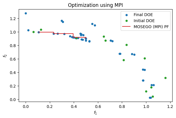
By default, MOSEGO uses the Expected Hypervolume Improvement (EHVI) acquisition function. However, other multi-objective enrichment criteria are available, such as the Minimum Probability of Improvement (MPI) (init_mpi).
You can easily switch the acquisition function by passing the strategy_kwargs={"acq_init": init_mpi} parameter to the Driver. The code cell below demonstrates how to optimize the same problem using MPI instead of EHVI.
from smt_optim.acquisition_functions import init_mpi

# Initialize the driver with MPI instead of EHVI
driver_mpi = Driver(prob_definition, opt_config, MOSEGO, strategy_kwargs={"acq_init": init_mpi})

# Start the optimization process
state_mpi = driver_mpi.optimize()

# Extract Pareto front
obj_mpi_par = get_pf_from_dataset(state_mpi.dataset)
sorted_idx_mpi = np.argsort(obj_mpi_par[:, 0])
obj_mpi_par = obj_mpi_par[sorted_idx_mpi, :]

# Plot the MPI Pareto front
fig, ax = plt.subplots(layout="constrained", figsize=(6, 4))
data_mpi = driver_mpi.state.dataset.export_as_dict()
obj_mpi = data_mpi["obj"]

ax.scatter(obj_mpi[nt_init:, 0], obj_mpi[nt_init:, 1], 20, color="C0", label="Final DOE")
ax.scatter(obj_mpi[:nt_init, 0], obj_mpi[:nt_init, 1], 20, color="C2", label="Initial DOE")
ax.step(obj_mpi_par[:, 0], obj_mpi_par[:, 1], where="post", color="C3", zorder=20, label="MOSEGO (MPI) PF")

ax.set_xlabel(r"$f_1$")
ax.set_ylabel(r"$f_2$")
ax.set_title("Optimization using MPI")
ax.legend()
plt.show()
          iter         budget             HV        spacing       fidelity        gp_time       acq_time
             0         16.800    2.01117e-01    0.00000e+00            nan            nan            nan
             1         17.000    2.01117e-01    0.00000e+00              1          6.618          5.441
             2         17.200    2.01117e-01    0.00000e+00              1          6.180          6.661
             3         17.400    2.01117e-01    0.00000e+00              1          6.595          7.366
             4         17.600    2.01117e-01    0.00000e+00              1          7.330          4.480
             5         17.800    2.01117e-01    0.00000e+00              1          6.246          7.126
             6         18.000    2.01117e-01    0.00000e+00              1          6.500          5.462
             7         18.200    2.01117e-01    0.00000e+00              1          6.325          6.827
             8         18.400    2.01117e-01    0.00000e+00              1          6.416          6.783
             9         19.600    2.05049e-01    5.18761e-02              2          6.467          5.453
          iter         budget             HV        spacing       fidelity        gp_time       acq_time
            10         19.800    2.05049e-01    5.18761e-02              1          6.494          5.567
            11         21.000    2.43620e-01    4.56394e-02              2          6.830          8.409
            12         21.200    2.43620e-01    4.56394e-02              1          6.752         13.562
            13         22.400    2.43983e-01    7.94352e-02              2          6.583          9.183
            14         22.600    2.43983e-01    7.94352e-02              1          6.712          5.464
            15         22.800    2.43983e-01    7.94352e-02              1          6.992          4.837
            16         24.000    2.53002e-01    7.06530e-02              2          6.648          7.256
            17         24.200    2.53002e-01    7.06530e-02              1          6.573          7.178
            18         24.400    2.53002e-01    7.06530e-02              1          7.375          7.592
            19         24.600    2.53002e-01    7.06530e-02              1          7.071          9.896
          iter         budget             HV        spacing       fidelity        gp_time       acq_time
            20         24.800    2.53002e-01    7.06530e-02              1          7.488          5.293